4/22/23

Data Engineering Process Fundamentals - Design and Planning Exercise

Having laid a strong design foundation, it's time to embark on a hands-on exercise that's crucial to our data engineering project's success. Our immediate focus is on building the essential cloud resources that will serve as the backbone for our data pipelines, data lake, and data warehouse. Taking a cloud-agnostic approach ensures our implementation remains flexible and adaptable across different cloud providers, enabling us to leverage the advantages of multiple platforms or switch providers seamlessly if required. By completing this step, we set the stage for efficient and effective coding of our solutions. Let's get started on this vital infrastructure-building journey.
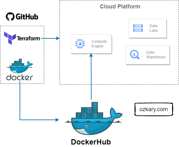
ozkary-data-engineering-design-planning-docker-terraform

Cloud Infrastructure Planning

Infrastructure planning is a critical aspect of every technical project, laying the foundation for successful project delivery. In the case of a Data Engineering project, it becomes even more crucial. To support our project's objectives, we need to carefully consider and provision specific resources:

  • VM instance: This serves as the backbone for hosting our data pipelines and orchestration, ensuring efficient execution of our data workflows.
  • Data Lake: A vital component for storing various data formats, such as CSV or Parquet files, in a scalable and flexible manner.
  • Data Warehouse: An essential resource that hosts transformed and curated data, providing a high-performance environment for easy access by visualization tools.

Infrastructure automation, facilitated by tools like Terraform, is important in modern data engineering projects. It enables the provisioning and management of cloud resources, such as virtual machines and storage, in a consistent and reproducible manner. Infrastructure as Code (IaC) allows teams to define their infrastructure declaratively, track it in source control, version it, and apply changes as needed. Automation reduces manual efforts, ensures consistency, and enables infrastructure to be treated as a code artifact, improving reliability and scalability.
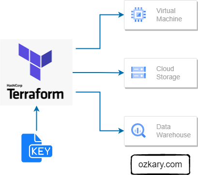
ozkary-data-engineering-terraform

Infrastructure Implementation Requirements

When using Terraform with a any cloud provider, there are several key artifacts and considerations to keep in mind for successful configuration and security. Terraform needs access to the cloud account where it can provision the resources. The account token or credentials can vary based on your cloud configuration. For our purpose, we will use a GCP (Google) project to build our resources, but first we need to install the Terraform dependencies for the development environment.

Install Terraform

To install Terraform, open a bash terminal and run the commands below:

  • Download the package file
  • Unzip the file
  • Copy the Terraform binary from the extracted file to the /usr/bin/ directory
  • Verify the version
$ wget https://releases.hashicorp.com/terraform/1.3.7/terraform_1.3.7_linux_amd64.zip
$ unzip terraform_1.1.2_linux_amd64.zip
$ cp terraform /usr/bin/
$ terraform -v

We should get an output similar to this:

Terraform v1.3.7
on linux_amd64

Configure a Cloud Account

Create a Google account. Here

  • Create a new project
  • Make sure to keep track of the Project ID and the location for your project

Create a service account

  • In the left-hand menu, click on "IAM & Admin" and then select "Service accounts"
  • Click on the "Create Service Account" button at the top of the page
  • Enter a name for the service account and an optional description
  • Then add the BigQuery Admin, Storage Admin, Storage Object Admin as roles for our service account and click the save button.

ozkary gcp roles

Authenticate the VM or Local environment with GCP

  • In the left navigation menu (GCP), click on "IAM & Admin" and then "Service accounts"
  • Click on the three verticals dots under the action section for the service name you just created
  • Then click Manage keys, Add key, Create new key. Select JSON option and click Create
  • Move the key file to a system folder
$ mkdir -p $HOME/.gcp/ 
$ mv ~/Downloads/{xxxxxx}.json ~/.gcp/{acc_credentials}.json
  • install the SDK and CLI Tools
  • Validate the installation and login to GCP with the following commands
    $ echo 'export GOOGLE_APPLICATION_CREDENTIALS="~/.gcp/{acc_credentials}.json"' >> ~/.bashrc
    $ export GOOGLE_APPLICATION_CREDENTIALS="~/.gcp/{acc_credentials}.json"
    $ gcloud auth application-default login
    
  • Follow the login process on the browser

Review the Code

👉 Clone this repo or copy the files from this folder

Terraform uses declarative configuration files written in a domain-specific language (DSL) called HCL (HashiCorp Configuration Language). It provides a concise and human-readable syntax for defining resources, dependencies, and configurations, enabling us to provision, modify, and destroy infrastructure in a predictable and reproducible manner.

At a minimum, we should define a variables file, which contains the cloud provider information and a resource file which define what kind of resources should be provision on the cloud. There could be a file for each resource or a single file can define multiple resources.

Variables File

The variables file is used to define a set of variables that can be used on the resource file. This allows for the use of those variables in one more more resource configuration files. The format looks as follows:

locals {
  data_lake_bucket = "mta_data_lake"
}

variable "project" {
  description = "Enter Your GCP Project ID"
  type = string
}

variable "region" {
  description = "Region for GCP resources. Choose as per your location: https://cloud.google.com/about/locations"
  default = "us-east1"
  type = string
}

variable "storage_class" {
  description = "Storage class type for your bucket. Check official docs for more info."
  default = "STANDARD"
  type = string
}

variable "stg_dataset" {
  description = "BigQuery Dataset that raw data (from GCS) will be written to"
  type = string
  default = "mta_data"
}

variable "vm_image" {
  description = "Base image for your Virtual Machine."
  type = string
  default = "ubuntu-os-cloud/ubuntu-2004-lts"
}

Resource File

The resource file is where we define what should be provisioned on the cloud. This is also the file where we need to define the provider specific resources that need to be created.

terraform {
  required_version = ">= 1.0"
  backend "local" {}  # Can change from "local" to "gcs" (for google) or "s3" (for aws), if you would like to preserve your tf-state online
  required_providers {
    google = {
      source  = "hashicorp/google"
    }
  }
}

provider "google" {
  project = var.project
  region = var.region
  // credentials = file(var.credentials)  # Use this if you do not want to set env-var GOOGLE_APPLICATION_CREDENTIALS
}

# Data Lake Bucket
# Ref: https://registry.terraform.io/providers/hashicorp/google/latest/docs/resources/storage_bucket
resource "google_storage_bucket" "data-lake-bucket" {
  name          = "${local.data_lake_bucket}_${var.project}" # Concatenating DL bucket & Project name for unique naming
  location      = var.region

  # Optional, but recommended settings:
  storage_class = var.storage_class
  uniform_bucket_level_access = true

  versioning {
    enabled     = true
  }

  lifecycle_rule {
    action {
      type = "Delete"
    }
    condition {
      age = 15  // days
    }
  }

  force_destroy = true
}

# BigQuery data warehouse
# Ref: https://registry.terraform.io/providers/hashicorp/google/latest/docs/resources/bigquery_dataset
resource "google_bigquery_dataset" "stg_dataset" {
  dataset_id = var.stg_dataset
  project    = var.project
  location   = var.region
}

# VM instance
resource "google_compute_instance" "vm_instance" {
  name          = "mta-instance"
  project       = var.project
  machine_type  = "e2-standard-4"
  zone          = var.region

  boot_disk {
    initialize_params {
      image = var.vm_image
    }
  }

  network_interface {
    network = "default"

    access_config {
      // Ephemeral public IP
    }
  }
}

This Terraform file defines the infrastructure components to be provisioned on the Google Cloud Platform (GCP). It includes the configuration for the Terraform backend, required providers, and the resources to be created.

  • The backend section specifies the backend type as "local" for storing the Terraform state locally. It can be changed to "gcs" or "s3" for cloud storage if desired.
  • The required_providers block defines the required provider and its source, in this case, the Google Cloud provider.
  • The provider block configures the Google provider with the project and region specified as variables. It can use either environment variable GOOGLE_APPLICATION_CREDENTIALS or the credentials file defined in the variables.
  • The resource blocks define the infrastructure resources to be created, such as a Google Storage Bucket for the data lake, Google BigQuery datasets for staging and production, and a Google Compute Engine instance named "mta-instance" with specific configuration settings.

Overall, this Terraform file automates the provisioning of a data lake bucket, BigQuery datasets, and a virtual machine instance on the Google Cloud Platform.

How to run it!

  • Refresh service-account's auth-token for this session
$ gcloud auth application-default login
  • Set the credentials file on the bash configuration file
    • Add the export line and replace filename-here with your file
$ echo export GOOGLE_APPLICATION_CREDENTIALS="${HOME}/.gcp/filename-here.json" >> ~/.bashrc && source ~/.bashrc
  • Open the terraform folder in your project

  • Initialize state file (.tfstate) by running terraform init

$ cd ./terraform
$ terraform init
  • Check changes to new infrastructure plan before applying them

It is important to always review the plan to make sure no unwanted changes are showing up.

👉 Get the project id from your GCP cloud console and replace it on the next command

$ terraform plan -var="project=<your-gcp-project-id>"
  • Apply the changes

This provisions the resources on the cloud project.

$ terraform apply -var="project=<your-gcp-project-id>"
  • (Optional) Delete infrastructure after your work, to avoid costs on any running services
$ terraform destroy

Terraform Lifecycle

ozkary-data-engineering-terraform-lifecycle

GitHub Action

In order to be able to automate the building of infrastructure with GitHub, we need to define the cloud provider token as a secret with GitHub. This can be done by following the steps from this link:

👉 Configure GitHub Secrets

Once the secret has been configured, we can create a build action script with the cloud provider secret information as shown with this GitHub Action workflow YAML file:


name: Terraform Deployment

on:
  push:
    branches:
      - main

jobs:
  deploy:
    runs-on: ubuntu-latest

    steps:
    - name: Checkout repository
      uses: actions/checkout@v2

    - name: Set up Terraform
      uses: hashicorp/setup-terraform@v1

    - name: Terraform Init
       env:        
        GOOGLE_APPLICATION_CREDENTIALS:  ${{ secrets.GOOGLE_APPLICATION_CREDENTIALS }}
      run: |
        cd Step2-Cloud-Infrastructure/terraform
        terraform init

    - name: Terraform Apply
      run: |
        cd path/to/terraform/project
        terraform apply -auto-approve

Conclusion

With this exercise, we gain practical experience in using tools like Terraform to automate the provisioning of resources, such as VM, a data lakes and other components essential to our data engineering system. By following cloud-agnostic practices, we can achieve interoperability and avoid vendor lock-in, ensuring our project remains scalable, cost-effective, and adaptable to future requirements.

Next Step

After building our cloud infrastructure, we are now ready to talk about the implementation and orchestration of a data pipeline and review some of the operational requirements that can enable us to make decisions.

Coming Soon!

👉 [Data Engineering Process Fundamentals - Data Pipeline and Orchestration]

Thanks for reading.

Send question or comment at Twitter @ozkary

👍 Originally published by ozkary.com

4/15/23

Data Engineering Process Fundamentals - Design and Planning

Now that we have completed the discovery step and the scope of work on the project is clearly defined, we move on to the design and planning step. The design and planning phase of a data engineering project is crucial for laying out the foundation of a successful system. It involves defining the system architecture, designing data pipelines, implementing source control practices, ensuring continuous integration and deployment (CI/CD), and leveraging tools like Docker and Terraform for infrastructure automation.

ozkary-data-engineering-design-planning

Data Engineering Design

A data engineering design is the actual plan to build the technical solution. It includes the system architecture, data integration, flow and pipeline orchestration, the data storage platform, transformation and management, data processing and analytics tooling. This is the area where we need to clearly define the different technologies that should be used for each area.

System Architecture

The system architecture is a critical high-level design that encompasses various components and their integration within the solution. This includes data sources, data ingestion resources, workflow and data orchestration frameworks, storage resources, data services for transformation, continuous data ingestion, and validation, as well as data analysis and visualization tools. Properly designing the system architecture ensures a robust and efficient data engineering solution.

Data Pipelines

A data pipeline refers to a series of connected tasks that handles the extract, transform and load (ETL) as well as the extract, load and transform (ELT) operations and integration from a source to a target storage like a data lake or data warehouse. Properly designed pipelines ensure data integrity, quality, and consistency throughout the system.

The use of ETL or ELT depends on the design. For some solutions, a flow task may transform the data prior to loading it into storage. This approach tends to increase the amount of python code and hardware resources used by the hosting environment. For the ELT process, the transformation may be done using SQL code and the data warehouse resources, which often tend to perform great for big data scenarios.

Data Orchestration

Data orchestration refers to the automation, management and coordination of the data pipeline tasks. It involves the scheduling, workflows, monitoring and recovery of those tasks. The orchestration ensures the execution of those tasks, and it takes care of error handling, retry and the alerting of problems in the pipeline.

Source Control and Deployment

Source control is an essential practice for managing code and configuration files. Utilizing version control systems allows teams to collaborate effectively, track changes, and revert to previous states if necessary. It is important to properly define the tooling that should be used for source control and deployments automation. Source code should include the Python code, Terraform scripts, Docker files as well as any deployment automation scripts.

Source Control

Client side source control systems such as Git help in tracking and maintaining the source code for our projects. Cloud side systems such as GitHub should be used to enable the team to push their code and configuration changes to a remote repository, so it can be shared with other team members.

Continuous Integration and Continuous Delivery (CI/CD)

A remote code repository like GitHub also provides deployment automation pipelines that enable us to push changes to other environments for testing and finally production releases.

Continuous Integration (CI) is the practice to continuously integrate the code changes into the central repository, so it can be built and tested to validate the latest change and provide feedback in case of problems. Continuous Deployment (CD) is the practice to automate the deployment of the latest code builds to other environments like staging and production.

Docker Containers and Docker Hub

When deploying a new build, we need to also deploy the environment dependencies to avoid any run-time errors. Docker containers enable us to automate the management of the application by creating a self-contained environment with the build and its dependencies. A data pipeline can be built and imported into a container image, which should contain everything needed for the pipeline to reliably execute.

Docker Hub is a container registry which allows us to push our pipeline images into a cloud repository. The goal is to provide the ability to download those images from the repository as part of the new environment provisioning process.

Terraform for Cloud Infrastructure

Terraform is an Infrastructure as Code (IaC) tool that enables us to manage cloud resources across multiple cloud providers. By creating resource definition scripts and tracking them under version control, we can automate the creation, modification and deletion of resources. Terraform tracks the state of the infrastructure, so when changes are made, they can be applied to the environments as part of a CI/CD process.

ozkary-data-engineering-design-planning-docker-terraform

Data Analysis and Visualization Tools

The selection of an analytical and visualization tool is very important in any data engineering projects. Tools like Looker, Power Builder among others enable business to gain insights from their data by visualizing the information on easy to read dashboards. By selecting the right tool for the job, organizations can transform complex data into actionable insights, empowering users across the business to uncover valuable information and drive strategic outcomes.

Summary

The design and planning phase of a data engineering project sets the stage for success. From designing the system architecture and data pipelines to implementing source control, CI/CD, Docker, and infrastructure automation with Terraform, every aspect contributes to efficient and reliable deployment. Infrastructure automation, in particular, plays a critical role by simplifying provisioning of cloud resources, ensuring consistency, and enabling scalability, ultimately leading to a robust and manageable data engineering system.

Exercise - Infrastructure Planning and Automation

Having established a solid design foundation, it's time to put that into practice with a hands-on exercise. Our objective is to construct the necessary infrastructure that will serve as the hosting environment for our solution. Let's delve into the practical implementation to bring our data engineering project to life.

👉 Data Engineering Process Fundamentals - Design and Planning Exercise

Thanks for reading.

Send question or comment at Twitter @ozkary

👍 Originally published by ozkary.com
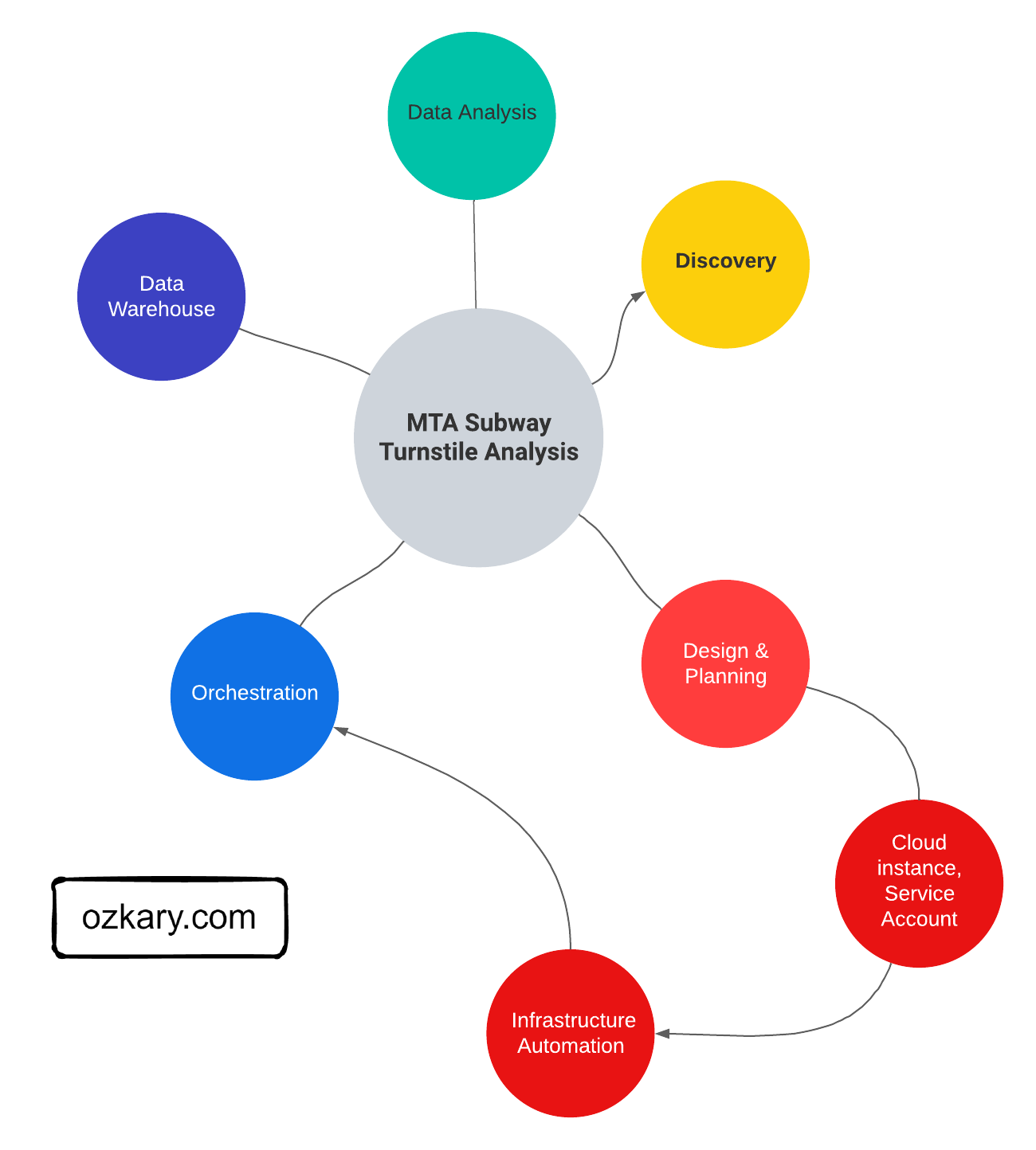
4/8/23

Data Engineering Process Fundamentals - Discovery Exercise

In this discovery exercise lab, we review a problem statement and do the analysis to define the scope of work and requirements.

Problem Statement

In the city of New York, commuters use the Metropolitan Transportation Authority (MTA) subway system for transportation. There are millions of people that use this system every day; therefore, businesses around the subway stations would like to be able to use Geofencing advertisement to target those commuters or possible consumers and attract them to their business locations at peak hours of the day.

Geofencing is a location based technology service in which mobile devices’ electronic signal is tracked as it enters or leaves a virtual boundary (geo-fence) on a geographical location. Businesses around those locations would like to use this technology to increase their sales.

ozkary-data-engineering-mta-geo-fence

The MTA subway system has stations around the city. All the stations are equipped with turnstiles or gates which tracks as each person enters or leaves the station. MTA provides this information in CSV files, which can be imported into a data warehouse to enable the analytical process to identify patterns that can enable these businesses to understand how to best target consumers.

Analytical Approach

Dataset Criteria

We are using the MTA Turnstile data for 2023. Using this data, we can investigate the following criteria:

  • Stations with the high number of exits by day and hours
  • Stations with high number of entries by day and hours

Exits indicates that commuters are arriving to those locations. Entries indicate that commuters are departing from those locations.

Data Analysis Criteria

The data can be grouped into stations, date and time of the day. This data is audited in blocks of fours hours apart. This means that there are intervals of 8am to 12pm as an example. We analyze the data into those time block intervals to help us identify the best times both in the morning and afternoon for each station location. This should allow businesses to target a particular geo-fence that is close to their business.

In the discovery process, we take a look at the data that is available for our analysis. We are using the MTA turnstiles information which is available at this location:

👉 New York Metropolitan Transportantion Authority Turnstile Data

We can download a single file to take a look at the data structure and make the following observations about the data:

Observations

  • It is available in weekly batches every Sunday
  • The information is audited in blocks of fours hours apart
  • The date and time field are on different columns
  • The cumulative entries are on the ENTRIES field
  • The cumulative exits are on the EXITS field
  • This data is audited in blocks of fours hours apart

ozkary-data-engineering-mta-discovery

Field Description

Name Description
C/A Control Area (A002) (Booth)
UNIT Remote Unit for a station (R051)
SCP Subunit Channel Position represents an specific address for a device (02-00-00)
STATION Represents the station name the device is located at
LINENAME Represents all train lines that can be boarded at this station. Normally lines are represented by one character. LINENAME 456NQR repersents train server for 4, 5, 6, N, Q, and R trains.
DIVISION Represents the Line originally the station belonged to BMT, IRT, or IND
DATE Represents the date (MM-DD-YY)
TIME Represents the time (hh:mm:ss) for a scheduled audit event
DESc Represent the “REGULAR” scheduled audit event (Normally occurs every 4 hours). Audits may occur more that 4 hours due to planning, or troubleshooting activities. Additionally, there may be a “RECOVR AUD” entry: This refers to missed audit that was recovered.
ENTRIES The cumulative entry register value for a device
EXIST The cumulative exit register value for a device

Data Example

The data below shows the entry/exit register values for one turnstile at control area (A002) from 09/27/14 at 00:00 hours to 09/29/14 at 00:00 hours

C/A UNIT SCP STATION LINENAME DIVISION DATE TIME DESC ENTRIES EXITS
A002 R051 02-00-00 LEXINGTON AVE 456NQR BMT 09-27-14 00:00:00 REGULAR 0004800073 0001629137
A002 R051 02-00-00 LEXINGTON AVE 456NQR BMT 09-27-14 04:00:00 REGULAR 0004800125 0001629149
A002 R051 02-00-00 LEXINGTON AVE 456NQR BMT 09-27-14 08:00:00 REGULAR 0004800146 0001629162

Conclusions

Based on observations, the following conclusions can be made:

  • Merge the DATE and TIME columns and create a date time column, CREATED
  • The STATION column is a location dimension
  • The CREATED column is the datetime dimension to enable the morning and afternoon timeframes
  • The ENTRIES column is the measure for entries
  • The EXITS column is the measure for exits
  • A gate can be identified by using the C/A, SCP and UNIT columns

Requirements

These observations can be used to define technical requirements that can enable us to deliver a successful project.

  • Define the infrastructure requirements to host the technology
    • Automate the provisioning of the resources using Terraform
    • Deploy the technology on a cloud platform
  • Define the data orchestration process
    • On the original pipeline, load the initial data for 2023
    • Create a data pipeline that runs every week after a new file has been published
    • Copy the unstructured CSV files into a Data Lake
  • Define a well-structured and optimized model on a Data Warehouse
    • Keep the source code for the models under source control
    • Copy the data into the Data Warehouse
    • Allow access to the Data Warehouse, so visualization tools can consume the data.
  • Create Data Analysis dashboard with the following information
    • Data Analysis dashboard
    • Identify the time slots for morning and afternoon analysis
    • Look at the distribution by stations
    • Look at the daily models
    • Look at the time slot models

Review the Code

In order to do our data analysis, we need to first download some sample data by writing a Python script. We can the analyze this data by writing some code snippets and use the power of the Python Pandas library. We can also use Jupyter Notebooks to quickly manipulate the data and create some charts that can help us as baseline requirements for the final visualization dashboard.

👉 Clone this repo or copy the files from this folder

Download a CSV File from the MTA Site

With this Python script (mta_discovery.py), we download a CSV file with the URL of http://web.mta.info/developers/data/nyct/turnstile/turnstile_230318.txt. The code creates a data stream to download the file in chunks to avoid any timeouts. We append the chunks into a local compressed file to reduce the size of the file. In order to reuse this code, we use the command line parser, so we can pass as parameters the URL.

import os
import argparse
from time import time
from pathlib import Path
import pandas as pd


def read_local(file_path: str) -> Path:
    """
        Reads a local file
        Args:
            file_path:  local file            
    """
    print(F'Reading local file {file_path}')
    df_iter = pd.read_csv(file_path, iterator=True,compression="gzip", chunksize=10000) 
    if df_iter:        
        for df in df_iter:
            try:                                
                print('File headers',df.columns)                                
                print('Top 10 rows',df.head(10))            
                break
            except Exception as ex:
                print(f"Error found {ex}")
                return

        print(f"file was loaded {file_path}")        
    else:
        print(F"failed to read file {file_path}")

def write_local(df: pd.DataFrame, folder: str, file_name: str) -> Path:
    """
        Write DataFrame out locally as csv file
        Args:
            df: dataframe chunk
            folder: the download data folder
            file_name: the local file name
    """

    path = Path(f"{folder}")
    if not os.path.exists(path):
        path.mkdir(parents=True, exist_ok=True)

    file_path = Path(f"{folder}/{file_name}")

    if not os.path.isfile(file_path):
        df.to_csv(file_path, compression="gzip")
        print('new file')
    else:
        df.to_csv(file_path, header=None, compression="gzip", mode="a")    
        print('chunk appended')

    return file_path

def etl_web_to_local(url: str, name: str) -> None:
    """
       Download a file    
       Args:
            url : The file url
            name : the file name

    """
    print(url, name)      

    # skip an existent file
    path = f"../data/"
    file_path = Path(f"{path}/{name}.csv.gz")
    if os.path.exists(file_path):
            read_local(file_path)            
            return

    df_iter = pd.read_csv(url, iterator=True, chunksize=10000) 
    if df_iter:      
        file_name = f"{name}.csv.gz"    
        for df in df_iter:
            try:                                                
                write_local(df, path, file_name)
            except StopIteration as ex:
                print(f"Finished reading file {ex}")
                break
            except Exception as ex:
                print(f"Error found {ex}")
                return

        print(f"file was loaded {file_path}")        
    else:
        print("dataframe failed")

def main_flow(params: str) -> None:
    """
        Process a CSV file from a url location with the goal to understand the data structure
    """    
    url = params.url  
    prefix = params.prefix

    try:
        start_index = url.index('_')
        end_index = url.index('.txt')
        file_name = F"{prefix}{url[start_index:end_index]}"
        # print(file_name)
        etl_web_to_local(url, file_name)
    except ValueError:
        print("Substring not found")


if __name__ == '__main__':

    os.system('clear')    
    parser = argparse.ArgumentParser(description='Process CSV data to understand the data')
    parser.add_argument('--url', required=True, help='url of the csv file')
    parser.add_argument('--prefix', required=True, help='the file prefix or group name')
    args = parser.parse_args()

    print('running...')
    main_flow(args)
    print('end')

Analyze the Data

With some sample data, we can now take a look at the data and make some observations. There are a few ways to approach the analysis. We could create another Python script and play with the data, but this will require to run the script from the console after every code change. A more productive way is to use Jupyter Notebooks. This tools enables us to edit and run code snippets in cells without having to run the entire script. This is a friendlier analysis tool that can help us focus on the data analysis instead of coding and running the script. In addition, once we are good with our changes, the notebook can be exported into a Python file. Let's look at that file discovery.ipynb:

import os
import argparse
from time import time
from pathlib import Path
import pandas as pd 

# read the file and display the top 10 rows
df = pd.read_csv('../data/230318.csv.gz', iterator=False,compression="gzip")
df.head(10)

# Create a new DateTime column and merge the DATE and TIME columns
df['CREATED'] =  pd.to_datetime(df['DATE'] + ' ' + df['TIME'], format='%m/%d/%Y %H:%M:%S')
df = df.drop('DATE', axis=1).drop('TIME',axis=1)
df.head(10)

# Aggregate the information by station and datetime
df["ENTRIES"] = df["ENTRIES"].astype(int)
df["EXITS"] = df["EXITS"].astype(int)
df_totals = df.groupby(["STATION","CREATED"], as_index=False)[["ENTRIES","EXITS"]].sum()
df_totals.head(10)

df_station_totals = df.groupby(["STATION"], as_index=False)[["ENTRIES","EXITS"]].sum()
df_station_totals.head(10)

# Show the total entries by station, use a subset of data
import plotly.express as px
import plotly.graph_objects as go

df_stations =  df_station_totals.head(25)
donut_chart = go.Figure(data=[go.Pie(labels=df_stations["STATION"], values=df_stations["ENTRIES"], hole=.2)])
donut_chart.update_layout(title_text='Entries Distribution by Station', margin=dict(t=40, b=0, l=10, r=10))
donut_chart.show()

# Show the data by the day of the week
df_by_date = df_totals.groupby(["CREATED"], as_index=False)[["ENTRIES"]].sum()
day_order = ['Sun', 'Mon', 'Tue', 'Wed', 'Thu', 'Fri', 'Sat']
df_by_date["WEEKDAY"] = pd.Categorical(df_by_date["CREATED"].dt.strftime('%a'), categories=day_order, ordered=True)
df_entries_by_date =  df_by_date.groupby(["WEEKDAY"], as_index=False)[["ENTRIES"]].sum()
df_entries_by_date.head(10)

bar_chart = go.Figure(data=[go.Bar(x=df_entries_by_date["WEEKDAY"], y=df_entries_by_date["ENTRIES"])])
bar_chart.update_layout(title_text='Total Entries by Week Day')
bar_chart.show()

How to Run it!

With an understanding of the code and tools, let's run the process.

Requirements

👉 Install Python, Pandas and Jupyter notebook

👉 Install Visual Studio Code

👉 Clone this repo or copy the files from this folder

Follow these steps to run the analysis

  • Download a file to look at the data
    • This should create a gz file under the ../data folder
$ python3 mta_discovery.py --url http://web.mta.info/developers/data/nyct/turnstile/turnstile_230318.txt

Run the Jupyter notebook (dicovery.ipynb) to do some analysis on the data.

  • Load the Jupyter notebook to do analysis
    • First start the Jupyter server from the terminal
$ jupyter notebook
  • See the URL on the terminal and click it to load it on the browser
    • Click the discovery.ipynb file link
  • Or open the file with VSCode and enter the URL when prompted from a kernel url
  • Run every cell from the top down as this is required to load the dependencies

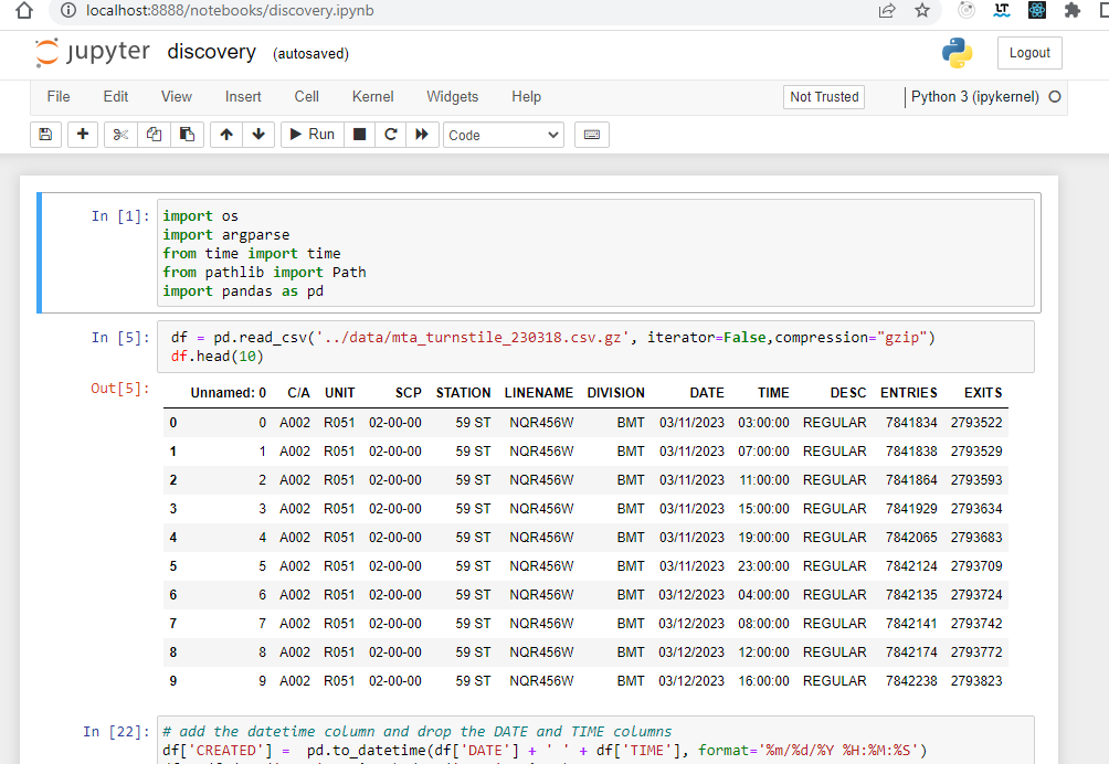
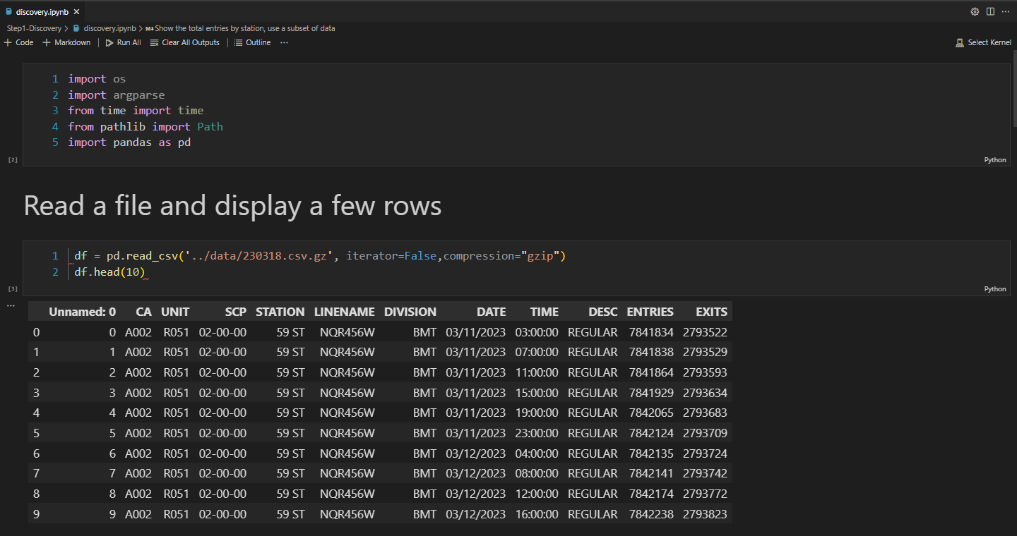
The following images show Jupyter notebook loaded on the browser or directly from VSCode.

Jupyter Notebook loaded on the browser

ozkary-data-engineering-jupyter-notebook

ozkary-data-engineering-discovery-query

Using VSCode to load the data and create charts

ozkary-data-engineering-discovery-jupyter-vscode

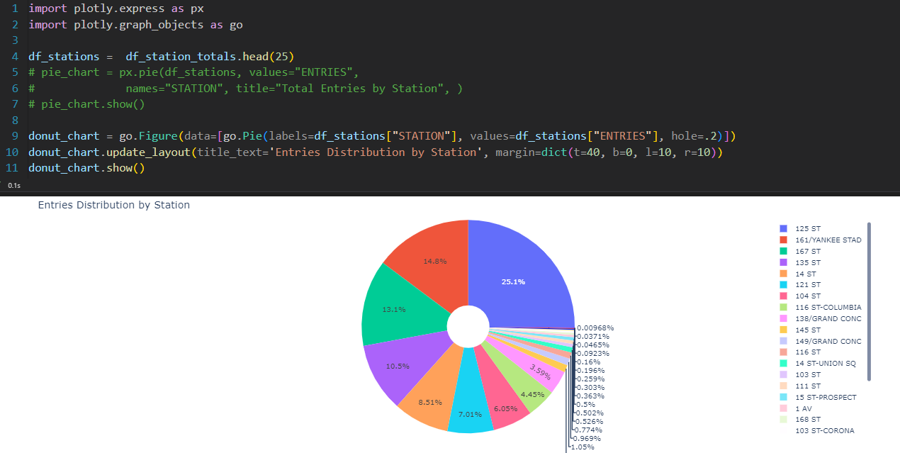
Show the total entries by station using a subset of data using VSCode

ozkary-data-engineering-discovery-donut-chart

Next Step

👉 Data Engineering Process Fundamentals - Design and Planning

Thanks for reading.

Send question or comment at Twitter @ozkary

👉 Originally published by ozkary.com

4/1/23

Data Engineering Process Fundamentals - Discovery

Introduction

In this series of Data Engineering Process Fundamentals, we explore the Data Engineering Process (DEP) with key concepts, principles and relevant technologies, and explain how they are being used to help us deliver solutions. The first step, and important to never skip, in this process is the Discovery step.

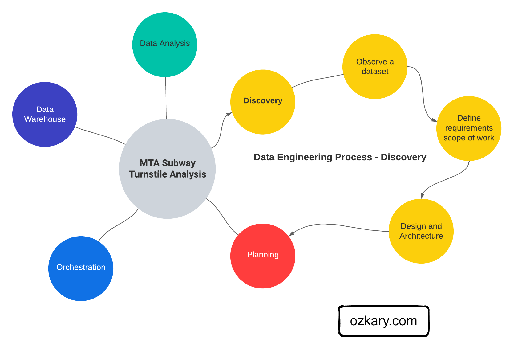
During the discovery step of a Data Engineering Process, we look to identify and clearly document a problem statement, which helps us have an understanding of what we are trying to solve. We also look at our analytical approach to make observations about at the data, its structure and source. This leads us into defining the requirements for the project, so we can define the scope, design and architecture of the solution.

ozkary-data-engineering-process-discovery

Problem Statement

A Problem Statement is a description of what it is that we are trying to solve. As part of the problem statement, we should provide some background or context on how the data is processed or collected. We should also provide a specific description of what the data engineering process is looking to solve by taking a specific approach to integrate the data. Finally, the objective and goals should also be described with information about how this data will be made available for analytical purposes.

Analytical Approach

The Analytical Approach is a systematic method to observe the data and arrive to insights from it. It involves the use of different techniques, tools and frameworks to make sense of the data in order to arrive to conclusions and actionable requirements.

Dataset Criteria

A Dataset Criteria technique refers to the set of characteristics used to evaluate the data, so we can determine the quality and accuracy of it.

In the data collection process, we should identify the various sources that can provide us with accurate and complete information. Data cleaning and preprocessing needs to be done to identify and eliminate missing values, invalid data and outliers that can skew the information. In addition, we should understand how this data is available for the ongoing integration. Some integrations may require a batch process integration at a scheduled interval. Others may require a real-time integration and/or a combination of batch and real-time processing.

Exploratory Data Analysis

We should conduct exploratory data analysis to understand the structure, patterns and characteristics of the data. We need to make observations about the data, identify the valuable fields, create statistical summaries, and run some data profiling to identify trends, metrics and correlations that are relevant to the main objective of the project.

Tools and Framework

Depending on the size and budget of the organization, the solution can be built with lots of coding and integration, or instead a low-code turn-key solution that provides enterprise quality resources could be used instead. Regardless of the approach, a programming language like Python is a popular programming language for data science and engineers, and it is always applicable. The Python Pandas library is great for data manipulation and analysis. Jupyter notes with Python scripts is great for experiments and discovery.

To run our Python scripts and Jupyter notebooks, we can use Visual Studio Code (VSCode), which is cross-platform Integrated Development Environment (IDE) tool. This tool also enables the integration with source control and deployments platforms like GitHub, so we can maintain version control and automate the deployment and test of our code changes.

To orchestrate the pipelines, we often use a workflow framework like Apache Airflow, Prefect. To host the data, we use data lakes (blob storage) and a relational data warehouse. For data modeling, incremental data and continuous test and data ingestion, Apache Spark or gbt cloud are used.

For the final data analysis and visualization, we could use tools like Looker, PowerBI and Tableau. These are tools that can connect to a data warehouse and consume the data models, so they can visualize in ways that enable stakeholders to make decisions based on the story provided by the data.

Requirements

Requirements refer to the needs, capabilities and constraints that are needed to deliver a data engineering solution. They should outline the project deliverables that are required to meet the main objectives. The requirements should include data related areas like:

  • Sources and integration
  • Modeling and transformation
  • Quality and validation
  • Storage and infrastructure
  • Processing and Analytics
  • Governance and Security
  • Scalability and performance
  • Monitoring

Design

A data engineering design is the actual plan to build the technical solution. It includes the system architecture, data integration, flow and pipeline orchestration, the data storage platform, transformation and management, data processing and analytics tooling. This is the area where we need to clearly define the different technologies that should be used for each area.

System Architecture

The system architecture is a high-level design of the solution, its components and how they integrate with each other. This often includes the data sources, data ingestion resources, workflow and data orchestration resources and frameworks, storage resources, data services for data transformation and continuous data ingestion and validation, and data analysis and visualization tooling.

Data Pipelines

A data pipeline refers to a series of connected tasks that handles the extract, transform and load (ETL) as well as the extract, load and transform (ELT) operations and integration from a source to a target storage like a data lake or data warehouse.

The use of ETL or ELT depends on the design. For some solutions, a flow task may transform the data prior to loading it into storage. This approach tends to increase the amount of python code and hardware resources used by the hosting environment. For the ELT process, the transformation may be done using SQL code and the data warehouse resources, which often tend to perform great for big data scenarios.

Data Orchestration

Data orchestration refers to the automation, management and coordination of the data pipeline tasks. It involves the scheduling, workflows, monitoring and recovery of those tasks. The orchestration ensures the execution of those tasks, and it takes care of error handling, retry and the alerting of problems in the pipeline.

Summary

The data engineering discovery process involves defining the problem statement, gathering requirements, and determining the scope of work. It also includes a data analysis exercise utilizing Python and Jupyter Notebooks ,or other tools, to extract valuable insights from the data. These steps collectively lay the foundation for successful data engineering endeavors.

Exercise - Hands-on Use Case

Since we now understand the discovery step, we should be able to put that into practice. Let’s move on to a hands-on use case and see how we apply those concepts.

👉 Data Engineering Process Fundamentals - Discovery Exercise

Thanks for reading.

Send question or comment at Twitter @ozkary

👍 Originally published by ozkary.com